

Autocorrelation
Basic Principle
Invented in the 1960’s, the optical autocorrelator was the first pulse measurement technique. As this technique is highly intuitive, many researchers, even now, use this technique, which measures the duration of a pulse directly. Figure 1 displays a schematic of a second harmonic generation (SHG) intensity autocorrelator. A beam splitter splits a pulse to be measured into two pulses, two replicas of the pulse, which are then focused onto an SHG crystal. The time delay between the two replicas is controlled by the length of a mechanical variable line. We can control the temporal overlapping of the two replicas in the SHG crystal. Depending on how much they overlap, the intensity of the SHG generated by the two replicas varies. We record the intensity as a function of the delay controlled by the delay line. In general, it can be done by a motorized translation stage.
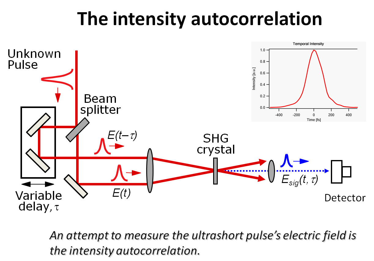
Figure 1: The schematic of an intensity autocorrelator. A beam splitter creates two replicas of the pulse to be measured. The variable delay moving stage can control the delay between the two replicas. If they overlap in the SHG crystal, they generate autocorrelation signals. The insert shows a typical autocorrelation trace. Note that the x-axis represents delay and the y-axis the normalized intensity..
Fig. 2 shows the procedure for estimating the length of a pulse with autocorrelation traces. The horizontal(X) axis represents the delay and the vertical (Y) axis the normalized intensity. To estimate the pulse duration, we must assume a pulse shape. If we assume the sech2-shaped pulses, the pulse duration could be ~0.65 times the width of the autocorrelation trace. If we assume a different pulse shape, the estimation would differ.
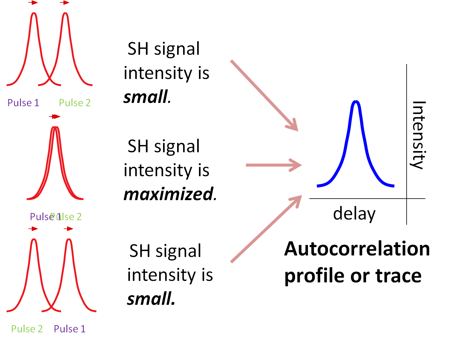
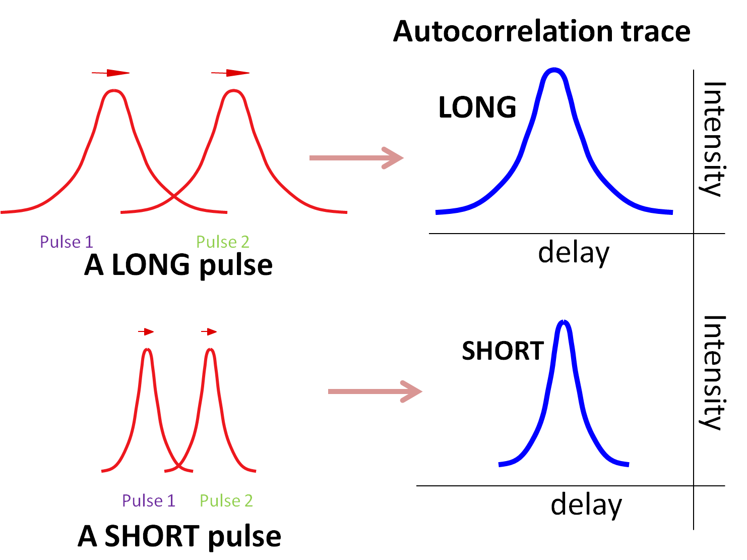
Figure 2: The SH signal intensity on the left-hand side varies, depending on how much the replicas overlap in time in the SHG crystal. When the replicas overlap perfectly in time, the SH signal intensity is maximized. The intensity is recorded as a function of the delay between the two replicas, as is an autocorrelation trace. On the right, a long pulse generates a wide trace and a short pulse a narrow trace. Therefore, it is possible to estimate the pulse duration.
Pros and Cons
The SHG crystal in an autocorrelator produces a signal at twice the frequency of the input pulse, and the detector measures the average power of the doubled frequency. Therefore, estimating the duration of a pulse does not require a fast photodetector. As autocorrelators always generate smooth and symmetric traces, however, it is impossible to see the temporal structure and/or the spectral structure of pulses, which could exist in pulses from fiber lasers or from not yet optimized oscillators. Furthermore, an extremely short pulse of less than 20fs could create a number of problems. We must use materials in the beam path, such as SHG crystal, lens and beam splitters, which would significantly stretch the pulses in the pulse duration. Phase-matching all the bandwidth of very short pulses requires an extremely thin crystal, which will considerably reduce the sensitivity of the device.
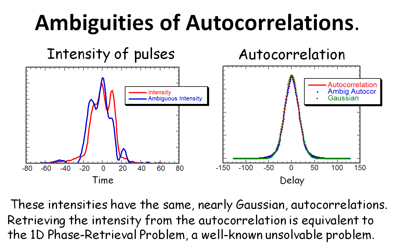
Figure 3: Results of simulation. Two different pulse intensities have the same, nearly Gaussian, autocorrelations. There are generally many ambiguous pulse intensities that generate the same autocorrelations. Note that even though the autocorrelation is smooth, the real pulse intensities have structures. Autocorrelation leads to considerable loss of information about the pulses. Therefore, the autocorrelation trace never allows us to know if the pulse has structures or not. Retrieving the intensity from the autocorrelation is equivalent to the 1D phase-retrieval problem, a well-known unsolvable problem. If you think a pulse has structures, or satellite pulses, autocorrelation is not an optimal technique for seeing the pulse.